Introduction

Chapter 7 of Machine Learning for Hackers is about numerical optimization. The authors organize the chapter around two examples of optimization. The first is a straightforward least-squares problem like that we’ve encountered already doing linear regressions, and is amenable to standard iterative algorithms (e.g. gradient descent). The second is a problem with a discrete search space, not clearly differentiable, and so lends itself to a stochastic/heuristic optimization technique (though we’ll see the optimization problem is basically artificial). The first problem gives us a chance to play around with Scipy’s optimization routines. The second problem has us hand-coding a Metropolis algorithm; this doesn’t show off much new Python, but it’s fun nonetheless.

The notebook for this chapter is at the github report here, or you can view it online via nbviewer here.

Ridge regression by least-squares

In chapter 6 we estimated LASSO regressions, which added an L1 penalty on the parameters to the OLS loss-function. The ridge regression works the same way, but applies an L2 penalty to the parameters. The ridge regression is a somewhat more straightforward optimization problem, since the L2 norm we use gives us a differentiable loss function.

In this example, we’ll regress weight on height, similar to chapter 5. We can specify the loss (sum of squared errors) function for the ridge regression with the following function in Python:

y = heights_weights['Weight'].values
Xmat = sm.add_constant(heights_weights['Height'], prepend = True)

def ridge_error(params, y, Xmat, lam):
    '''
    Compute SSE of the ridge regression.
    This is the normal regression SSE, plus the
    L2 cost of the parameters.
    '''
    predicted = np.dot(Xmat, params)
    sse = ((y - predicted) ** 2).sum()
    sse += lam * (params ** 2).sum()

    return sse

The authors use R’s optim function, which defaults to the Nelder-Mead simplex algorithm. This algorithm doesn’t use any gradient or Hessian information to optimize the function. We’ll want to try out some gradient methods, though. Even though the functions for these methods will compute numerical gradients and Hessians for us, for the ridge problem these are easy enough to specify explicitly.

def ridge_grad(params, y, Xmat, lam):
    '''
    The gradiant of the ridge regression SSE.
    '''
    grad = np.dot(np.dot(Xmat.T, Xmat), params) - np.dot(Xmat.T, y)
    grad += lam * params
    grad *= 2
    return grad

def ridge_hess(params, y, Xmat, lam):
'''
The hessian of the ridge regression SSE.
'''
    return np.dot(Xmat.T, Xmat) + np.eye(2) * lam

Like the LASSO regressions we worked with in chapter 6, the ridge requires a penalty parameter to weight the L2 cost of the coefficient parameters (called lam in the functions above; lambda is a keyword in Python). The authors assume we’ve already found an appropriate value via cross-validation, and that value is 1.0.

We can now try to minimize the loss function with a couple of different algorithms. First the Nelder-Mead simplex, which should correspond to the authors’ use of optim in R.

# Starting values for the a, b (intercept, slope) parameters
params0 = np.array([0.0, 0.0])

# Nelder-Mead simplex
ridge_fit = opt.fmin(ridge_error, params0, args = (y, Xmat, 1))
print 'Solution: a = %8.3f, b = %8.3f ' % tuple(ridge_fit)

Optimization terminated successfully.
Current function value: 1612442.197636
Iterations: 117
Function evaluations: 221
Solution: a = -340.565, b = 7.565

Now the Newton conjugate-gradient method. We need to give this function a gradient; the Hessian is optional. First without the Hessian:

ridge_fit = opt.fmin_ncg(ridge_error, params0, fprime = ridge_grad,
args = (y, Xmat, 1))
print 'Solution: a = %8.3f, b = %8.3f ' % tuple(ridge_fit)

Optimization terminated successfully.
Current function value: 1612442.197636
Iterations: 3
Function evaluations: 4
Gradient evaluations: 11
Hessian evaluations: 0
Solution: a = -340.565, b = 7.565

Now supplying the Hessian:

ridge_fit = opt.fmin_ncg(ridge_error, params0, fprime =
ridge_grad,
fhess = ridge_hess, args = (y, Xmat, 1))
print 'Solution: a = %8.3f, b = %8.3f ' % tuple(ridge_fit)

Optimization terminated successfully.
Current function value: 1612442.197636
Iterations: 3
Function evaluations: 7
Gradient evaluations: 3
Hessian evaluations: 3
Solution: a = -340.565, b = 7.565

Fortunately, we get the same results for all three methods. Supplying the Hessian to the Newton method shaves some time off, but in this simple application, it’s not really worth coding up a Hessian function (except for fun).

Lastly, the BFGS method, supplied with the gradient:

ridge_fit = opt.fmin_ncg(ridge_error, params0, fprime = ridge_grad,
fhess = ridge_hess, args = (y, Xmat, 1))
print 'Solution: a = %8.3f, b = %8.3f ' % tuple(ridge_fit)

Optimization terminated successfully.
Current function value: 1612442.197636
Iterations: 3
Function evaluations: 7
Gradient evaluations: 3
Hessian evaluations: 3
Solution: a = -340.565, b = 7.565

For this simple problem, all of these methods work well. For more complicated problems, there are considerations which would lead you to prefer one over another, or perhaps to use them in combination. There are also several more methods available, some which allow you to solve constrained optimization problems. Check out the very good documentation. Also note that if you’re not into hand-coding gradients, scipy has a function derivative in its misc module that will compute numerical derivatives. In many cases, the functions will do this automatically if you fail to provide a function to their gradient arguments.

Optimizing on sentences with the Metropolis algorithm

The second example in this chapter is a “code-breaking” exercise. We start with a message “here is some sample text”, which we encrypt using a Ceasar cipher that shifts each letter in the message to the next letter in the alphabet (with Z going to A). We can represent the cipher (or any cipher) in Python with a dict that maps each letter to its encrypted counterpart.

letters = ['a', 'b', 'c', 'd', 'e', 'f', 'g', 'h',
           'i', 'j', 'k', 'l', 'm', 'n', 'o', 'p',
           'q', 'r', 's', 't', 'u', 'v', 'w', 'x',
           'y', 'z']

ceasar_cipher = {i: j for i, j in zip(letters, letters[1:] + letters[:1])}
inverse_ceasar_cipher = {ceasar_cipher[k]: k for k in ceasar_cipher}

The inverse_ceasar_cipher dict reverses the cipher, so we can get an original message back from one that’s been encrypted by the Ceasar cipher. Based on these structures, let’s make functions that will encrypt and decrypt text.

def cipher_text(text, cipher_dict = ceasar_cipher):
    # Split the string into a list of characters to apply
    # the decoder over.
    strlist = list(text)

    ciphered = ''.join([cipher_dict.get(x) or x for x in strlist])
    return ciphered

def decipher_text(text, cipher_dict = ceasar_cipher):
    # Split the string into a list of characters to apply
    # the decoder over.
    strlist = list(text)

    # Invert the cipher dictionary (k, v) -> (v, k)
    decipher_dict = {cipher_dict[k]: k for k in cipher_dict}

    deciphered = ''.join([decipher_dict.get(x) or x for x in strlist])
    return deciphered

To decrypt our message, we’ll design a Metropolis algorithm that randomly proposes ciphers, decrypts the message according to the proposed cipher, and see’s how probable that message is based on a lexical database of word frequency in Wikipedia.

The following functions are used to generate proposal ciphers for the Metropolis algorithm. The idea is to randomly generate ciphers and see what text they result in. If the text resulting from a proposed cipher is more likely (according to the lexical database) than the current cipher, we accept the proposal. If it’s not, we accept it wil a probability that is lower the less likely the resulting text is.

The method of generating new proposals is important. The authors use a method that chooses a key (letter) at random from the current cipher, and swaps its with some other letter. For example, if we start with the Ceasar Cipher, our proposal might randomly choose to re-map A to N (instead of B). The proposal would then be the same a the Ceasar Cipher, but with A → N and M → B (since A originally mapped to B and M originally mapped to N). This proposal-generating mechanism is encapsulated in propose_modified_cipher_from_cipher.

This is inefficient in a few ways. First, the letter chosen to modify in the cipher may not even appear in the text, so the proposed cipher won’t modify the text at all and you end up wasting cycles generating a lot of useless proposals. Second, we may end up picking a letter that occurs in a highly likely word, which will increase the probability of generating an inferior proposal.

We’ll suggest another mechanism that, instead of selecting a letter from the current cipher to re-map, will choose a letter amongst the non-words in the current deciphered text. For example, if our current deciphered text is “hello wqrld”, we will only select amongst {w, q, r, l, d} to modify at random. The minimizes the chances that a modified cipher will turn real words into gibberish and produce less likely text. The function propose_modified_cipher_from_text performs this proposal mechanism.

One way to think of this is that it’s analogous to tuning the variance of the proposal distribution in the typical Metropolis algorithm. If the variance is too low, our algorithm won’t efficiently explore the target distribution. If it’s too high, we’ll end up generating lots of lousy proposals. Our cipher proposal rules can suffer from similar problems.

def generate_random_cipher():
    '''
    Randomly generate a cipher dictionary (a one-to-one letter -> letter
    map).
    Used to generate the starting cipher of the algorithm.
    '''
    cipher = []

    input = letters
    output = letters[:]
    random.shuffle(output)

    cipher_dict = {k: v for (k, v) in zip(input, output)}

    return cipher_dict

def modify_cipher(cipher_dict, input, new_output):
    '''
    Swap a single key in a cipher dictionary.

    Old: a -> b, ..., m -> n, ...
    New: a -> n, ..., m -> b, ...
    '''
    decipher_dict = {cipher_dict[k]: k for k in cipher_dict}
    old_output = cipher_dict[input]

    new_cipher = cipher_dict.copy()
    new_cipher[input] = new_output
    new_cipher[decipher_dict[new_output]] = old_output

    return new_cipher

def propose_modified_cipher_from_cipher(text, cipher_dict,
                                        lexical_db = lexical_database):
    '''
    Generates a new cipher by choosing and swapping a key in the
    current cipher.
    '''
    _ = text # Unused
    input = random.sample(cipher_dict.keys(), 1)[0]
    new_output = random.sample(letters, 1)[0]
    return modify_cipher(cipher_dict, input, new_output)

    def propose_modified_cipher_from_text(text, cipher_dict,
    lexical_db = lexical_database):

    '''
    Generates a new cipher by choosing a swapping a key in the current
    cipher, but only chooses keys that are letters that appear in the
    gibberish words in the current text.
    '''
    deciphered = decipher_text(text, cipher_dict).split()
    letters_to_sample = ''.join([t for t in deciphered
    if lexical_db.get(t) is None])
    letters_to_sample = letters_to_sample or ''.join(set(deciphered))

    input = random.sample(letters_to_sample, 1)[0]
    new_output = random.sample(letters, 1)[0]
    return modify_cipher(cipher_dict, input, new_output)

Next, we need to be able to compute a message’s likelihood (from the lexical database). The log-likelihood of a message is just the sum of the log-likelihoods of each word (one-gram) in the message. If the word is gibberish (i.e., doesn’t occur in the database) it gets a tiny probability set to the smallest floating-point precision.

def one_gram_prob(one_gram, lexical_db = lexical_database):
    return lexical_db.get(one_gram) or np.finfo(float).eps

    def text_logp(text, cipher_dict, lexical_db = lexical_database):
    deciphered = decipher_text(text, cipher_dict).split()
    logp = np.array([math.log(one_gram_prob(w)) for w in
    deciphered]).sum()
    return logp

We can now use these functions in our Metropolis algorithm. Each step in the metropolis algorithm proposes a cipher, deciphers the text according the proposal, and computes the log-likelihood of the deciphered message. If the likelihood of the deciphered message is better under the proposal cipher than the current cipher, we definitely accept that proposal for our next step. If not, we only accept the proposal with a probability based on the relative likelihood of the proposal to the current cipher.

I’ll define this function to take an arbitrary proposal function via the proposal_rule argument. So far, this can be one of the two propose_modified_cipher_from_* functions defined above.

def metropolis_step(text, cipher_dict, proposal_rule, lexical_db =
    lexical_database):
    proposed_cipher = proposal_rule(text, cipher_dict)
    lp1 = text_logp(text, cipher_dict)
    lp2 = text_logp(text, proposed_cipher)

    if lp2 > lp1:
        return proposed_cipher
    else:
        a = math.exp(lp2 - lp1)
        x = random.random()
        if x < a:
            return proposed_cipher
        else:
            return cipher_dict

To run the algorithm, just wrap the step function inside a loop. There’s no stopping rule for the algorithm, so we have to choose a number of iterations, and hope it’s enough to get us to the optimum. Let’s use 250,000.

message = 'here is some sample text'
ciphered_text = cipher_text(message, ceasar_cipher)
niter = 250000

def metropolis_decipher(ciphered_text, proposal_rule, niter, seed = 4):
    random.seed(seed)
    cipher = generate_random_cipher()

    deciphered_text_list = []
    logp_list = []

    for i in xrange(niter):
    logp = text_logp(ciphered_text, cipher)
    current_deciphered_text = decipher_text(ciphered_text, cipher)

    deciphered_text_list.append(current_deciphered_text)
    logp_list.append(logp)

    cipher = metropolis_step(ciphered_text, cipher, proposal_rule)

    results = DataFrame({'deciphered_text': deciphered_text_list, 'logp':
    logp_list})
    results.index = np.arange(1, niter + 1)
    return results

First let’s look at the authors’ proposal rule. While they managed to get a reasonable decrypted message in about 50,000 iterations, we’re still reading gibberish after 250,000. As they say in the book, their results are an artefact of a lucky seed value.

results0 = metropolis_decipher(ciphered_text,
propose_modified_cipher_from_cipher, niter)
print results0.ix[10000::10000]

               deciphered_text       logp
 10000 kudu of feru fyrvbu hush -86.585205
 20000 wudu of feru fbrkxu hush -87.124919
 30000 kudu of feru fnrbau hush -86.585205
 40000 wudu of feru fmrjiu hush -87.124919
 50000 kudu of feru fyrnbu hush -86.585205
 60000 kudu of feru fxrnvu hush -86.585205
 70000 pudu of feru fvrnlu hush -87.561022
 80000 kudu of feru fvrxgu hush -86.585205
 90000 kudu of feru fbrvtu hush -86.585205
100000 kudu of feru fjrnlu hush -86.585205
110000 kudu of feru fprbju hush -86.585205
120000 kudu of feru fnrjcu hush -86.585205
130000 kudu of feru flrvpu hush -86.585205
140000 puku of feru flrvxu hush -88.028362
150000 kudu of feru fxrviu hush -86.585205
160000 pulu of feru ftrdzu hush -88.323162
170000 wuzu of feru flrxdu hush -89.575925
180000 kudu of feru firamu hush -86.585205
190000 wudu of feru fyrzqu hush -87.124919
200000 wudu of feru fnraxu hush -87.124919
210000 puku of feru fjrnyu hush -88.028362
220000 puku of feru firyau hush -88.028362
230000 pudu of feru fkrcvu hush -87.561022
240000 kudu of feru ftrwzu hush -86.585205
250000 kudu of feru fprxzu hush -86.585205

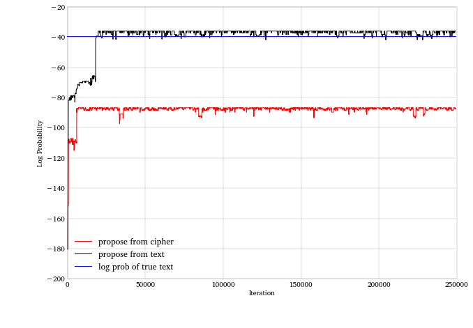
Now, let’s try the alternative proposal rule, which only chooses letters from gibberish words when it modifies the current cipher to propose a new one. The algorithm doesn’t find the actual message, but it actually finds a more likely message (according the the lexical database) within 20,000 iterations.

results1 = metropolis_decipher(ciphered_text,
propose_modified_cipher_from_text, niter)
print results1.ix[10000::10000]

                deciphered_text       logp
 10000 were mi isle izlkde text -68.946850
 20000 were as some simple text -35.784429
 30000 were as some simple text -35.784429
 40000 were as some simple text -35.784429
 50000 were as some simple text -35.784429
 60000 were as some simple text -35.784429
 70000 were us some simple text -38.176725
 80000 were as some simple text -35.784429
 90000 were as some simple text -35.784429
100000 were as some simple text -35.784429
110000 were as some simple text -35.784429
120000 were as some simple text -35.784429
130000 were as some simple text -35.784429
140000 were as some simple text -35.784429
150000 were us some simple text -38.176725
160000 were as some simple text -35.784429
170000 were is some sample text -37.012894
180000 were as some simple text -35.784429
190000 were as some simple text -35.784429
200000 were as some simple text -35.784429
210000 were as some simple text -35.784429
220000 were as some simple text -35.784429
230000 were as some simple text -35.784429
240000 were as some simple text -35.784429
250000 were is some sample text -37.012894

The graph below plots the likelihood paths of the algorithm for the two proposal rules. The blue line is the log-likelihood of the original message we’re trying to recover.

Direct calculation of the most likely message

The Metropolis algorithm is kind of pointless for this application. It’s really just jumping around looking for the most likely phrase. But since the likelihood of a message is just the sum of the log probabilities of the log probabilities of its component words, we just need to look for the most likely words of the lengths of the words of the ciphered message.

If the message at some point is “fgk tp hpdt”, then, if run long enough, the algorithm should just find the most likely three-letter word, the most likely two-letter word, and the most likely four-letter word. But we can look these up directly.

For example, the message we encrypted is ‘here is some sample text’, which has word lengths 4, 2, 4, 6, 4. What’s the most likely message with these word lengths?

def maxprob_message(word_lens = (4, 2, 4, 6, 4), lexical_db =
lexical_database):
    db_word_series = Series(lexical_db.index)
    db_word_len = db_word_series.str.len()
    max_prob_wordlist = []
    logp = 0.0
    for i in word_lens:
        db_words_i = list(db_word_series[db_word_len == i])
        db_max_prob_word = lexical_db[db_words_i].idxmax()
        logp += math.log(lexical_db[db_words_i].max())
        max_prob_wordlist.append(db_max_prob_word)
    return max_prob_wordlist, logp

maxprob_message()


(['with', 'of', 'with', 'united', 'with'], -25.642396806584493)

So, technically, we should have decoded our message to be “with of united with” instead of “here is some sample text”. This is not a shining endorsement of this methodology for decrypting messages.

Conclusion

While it was a fun exercise to code up the Metropolis decrypter in this chapter, it didn’t show off any new Python functionality. The ridge problem, while less interesting, showed off some of the optimization algorithms in Scipy. There’s a lot of good stuff in Scipy’s optimize module, and its documentation is worth checking out.