In my opinion, Chapter 6 is the most important chapter in Machine Learning for Hackers. It introduces the fundamental problem of machine learning: overfitting and the bias-variance tradeoff. And it demonstrates the two key tools for dealing with it: regularization and cross-validation.

It’s also a fun chapter to write in Python, because it lets me play with the fantastic scikit-learn library. scikit-learn is loaded with hi-tech machine learning models, along with convenient “pipeline”-type functions that facilitate the process of cross-validating and selecting hyperparameters for models. Best of all, it’s very well documented.

Fitting a sine wave with polynomial regression

The chapter starts out with a useful toy example—trying to fit a curve to data generated by a sine function over the interval [0, 1] with added Gaussian noise. The natural way to fit nonlinear data like this is using a polynomial function, so that the output, y is a function of powers of the input x. But there are two problems with this.

First, we can generate highly correlated regressors by taking powers of x, leading to noisy parameter estimates. The input x are evenly space numbers on the interval [0, 1]. So x and x² are going to have a correlation over 95%. Similar with x² and x³. The solution to this is to use orthogonalized polynomial functions: tranformations of x that, when summed, result in polynomial functions, but are orthogonal (therefore uncorrelated) with each other.

Luckily, we can easily calculate these transformations using patsy. The C(x, Poly) transform computes orthonormal polynomial functions of x, then we’ll extract out various orders of the polynomial. So Xpoly[:, :2] selects out the 0th and 1st order functions, then when summed will give us a first order polynomial (i.e. linear). Similarly Xpoly[: :4] gives us the 0th through 3rd order functions, which sum up to a cubic polynomial.

sin_data = DataFrame({'x' : np.linspace(0, 1, 101)})
sin_data['y'] = np.sin(2 \* pi \* sin_data['x']) +
np.random.normal(0, 0.1, 101)

x = sin_data['x']
y = sin_data['y']
Xpoly = dmatrix('C(x, Poly)')
Xpoly1 = Xpoly[:, :2]
Xpoly3 = Xpoly[:, :4]
Xpoly5 = Xpoly[:, :6]
Xpoly25 = Xpoly[:, :26]

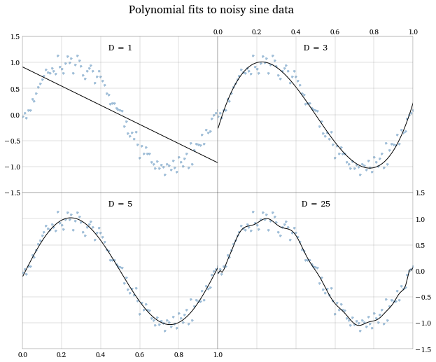
The problem we encounter now is how to choose what order polynomial to fit to the data. Any data can be fit well (i.e. have a high R^2^) if we use a high enough order polynomial. But we will start to over-fit our data; capturing noise specific to our sample, leading to poor predictions on new data. The graph below shows the fits to the data of a straight line, a 3rd-order polynomial, a 5th-order polynomial, and a 25th-order polynomial. Notice how the last fit gives us all kinds of degrees of freedom to capture specific datapoints, and the excessive “wiggles” look like we’re fitting to noise.

In machine learning, this problem is solved with regularization—penalizing large parameter estimates in a way that, hopefully, shrinks down the coefficients on all but the most important inputs. Here’s where scikit-learn shines.

Preventing overfitting with regularization

The penalty parameter in a regularized regression is typically found via cross-validation; for each candidate penalty one repeatedly fits the model on subsets on the data, and the penalty value that gives the best fit across the cross-validation “folds” is chosen. In the book, the authors hand-code up a cross-validation scheme, looping over possible penalties and subsets of the data and recording the MSEs.

In scikit-learn you can usually automate the cross-validation procedure, by one of a couple of ways. Many models have a CVversion, or, if not, you can wrap your model in a function like GridSearchCV which is a convenience function around all the looping and fit-recording entailed in a cross-validation. Here I’ll use the LassoCV function, which performs cross-validation for a LASSO-penalized linear regression.

lasso_model = LassoCV(cv = 15, copy_X = True, normalize = True)
lasso_fit = lasso_model.fit(Xpoly[:, 1:11], y)
lasso_path = lasso_model.score(Xpoly[:, 1:11], y)

The first line sets up the model by specifying some options. The only interesting one here is cv, which specifies how many cross-validation folds to run on each penalty-parameter value. The second line fits the model: here’s I’m going to run a 10th-order polynomial regression, and let the LASSO penalty shrink away all but the most important orders. Finally, lasso_path provides the objective function that our penalty parameter is suppose to optimize in the cross-validations (typically RMSE).

After running the fit() method, LassoCV will provide useful output attributes, including the “optimal” penalty parameter, stored in .alpha_. Note that scikit-learn refers to the penalty parameter as alpha, while R’s glmnet, which the authors use to implement the LASSO model, calls it lambda. I’m more accustomed to the penalty parameter being denoted with lambda myself. Note also that glmnet uses alpha elsewhere.

# Plot the average MSE across folds
plt.plot(-np.log(lasso_fit.alphas_),
np.sqrt(lasso_fit.mse_path_).mean(axis = 1))
plt.ylabel('RMSE (avg. across folds)')
plt.xlabel(r'\$-\\log(\\lambda)\$')
# Indicate the lasso parameter that minimizes the average MSE across
folds.
plt.axvline(-np.log(lasso_fit.alpha_), color = 'red')

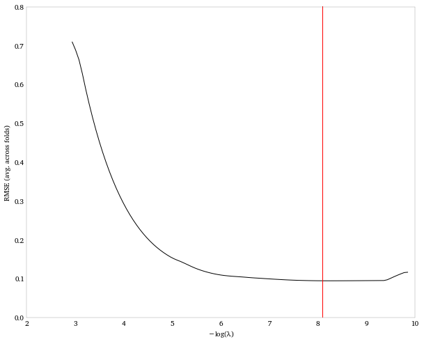
The value of the penalty parameter itself isn’t all that meaningful. So let’s take a look at what the resulting coefficient estimates are when we apply the penalty.

print 'Deg. Coefficient'
print Series(np.r_[lasso_fit.intercept_, lasso_fit.coef_])

Deg. Coefficient
  0    -0.003584
  1    -5.359452
  2     0.000000
  3     4.689958
  4    -0.000000
  5    -0.547131
  6    -0.047675
  7     0.124998
  8     0.133224
  9    -0.171974
 10     0.090685

So the LASSO, after selecting a penalty parameter via cross-validation, results in essentially a 3rd-order polynomial model: y = -5.4x + 4.7x^3^. This makes sense since, as we saw above, we’d captured the important features of the data by the time we’d fit a 3rd order polynomial.

Predicting O’Reilly book sales using back-cover descriptions

Next I’ll use the same model to tackle some real data. We have the sales ranks of the top-100 selling O’Reilly books. We’d like to see if we use the text on the back-cover description of the book to predict its rank. So the output variable is the rank of the book (reversed so that 100 is the top-selling book, and 1 is the 100th best-selling book), while the input variables are all the terms that appear in these 100 books’ back covers. For each book the value of an input variable is the number of times the term appears on its back cover. Many of the input values will be zero (for example, the term “javascript” will occur many times in a book about javascript, but zero times in every other book).

So the matrix of input variables is just our old friend, the term-document matrix. Creating this (using any of the methods described in the posts for [chapter 3][] or [chapter 4][]), we can just apply LassoCV again.

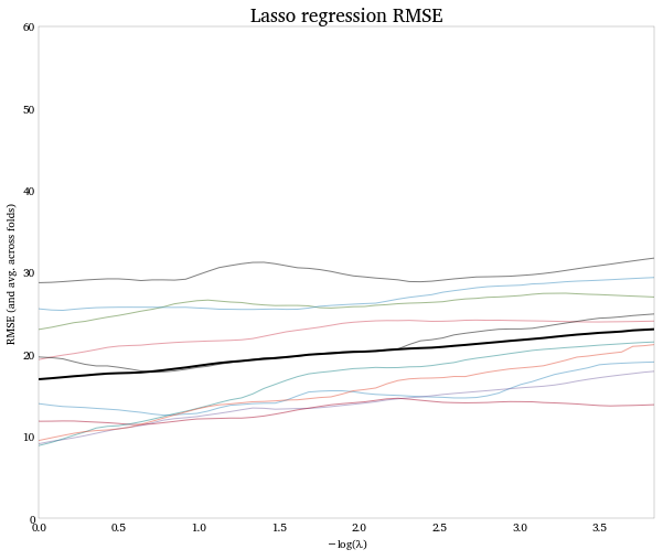
lasso_model = LassoCV(cv = 10)
lasso_fit = lasso_model.fit(desc_tdm.values, ranks.values)

Because of the size and nature of the input data, this runs pretty slowly (about 3-5 minutes for me). And, because there seems to be no good prediction model to be had here, the model doesn’t alway converge. If we do get a convergent run, we find the CV procedure wants us to shrink all the coefficients to zero: no input is worth keeping per the LASSO. (Note that since the x-axis in the graph is -log(penalty), moving left on the axis, towards 0, means more regularization.) This is the same result the authors find.

Logistic regression with cross-validation

With the previous model a bust, the authors regroup and try to fit a more simple output variable: a binary indicator of whether the book is in the top-50 sellers or not. Since they’re modeling a 0/1 outcome, they use a logistic regression. Like the linear models we used above, we can also apply regularizers to logistic regression.

In the book, the authors again code up an explicit cross-validation procedure. The notebook for this chapter has some code that replicates their procedure, but here I’ll discuss a version that uses scikit-learn’s GridCV function, which automates the cross-validation procedure for us. (the term “grid” is a little confusing here, since we’re only optimizing over one variable, the penalty parameter; the term “grid” is a little more intuitive in a 2-or-more-dimension search).

clf = GridSearchCV(LogisticRegression(C = 1.0, penalty = 'l1'),
c_grid,
score_func = metrics.zero_one_score, cv = n_cv_folds)
clf.fit(trainX, trainy)

We initialize the GridCV procedure by telling it:

• What model we’re using: logistic, with a penalty parameter C, initialized at 1.0, using the L1 (LASSO) penalty.
• A grid/array of parameter value candidates to search over: here values of C.
• A score function to optimize: before we were using the RMSE of the regression, here we’ll use a correct classification rate, given by zero_one_score, in scikit-learn’s metrics module.
• The number of cross-validation folds to performs; this defined elsewhere in the variable n_cv_folds

Then I fit the model on training data (a random subset of 80). After running this, We can check what value it chose for the penalty parameter, C, and what the in-sample error-rate for this value was.

clf.best_params_, 1.0 - clf.best_score_
({'C': 0.29377144516536563}, 0.375)

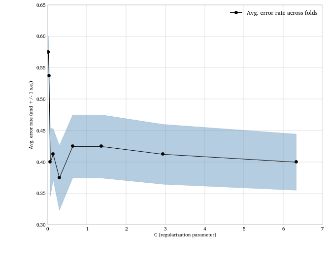
And again, let’s plot the error rates against values of C to vizualize how regularization affects the model accuracy.

rates = np.array([1.0 - x[1] for x in clf.grid_scores_])
stds = [np.std(1.0 - x[2]) / math.sqrt(n_cv_folds) for x in
clf.grid_scores_]

plt.fill_between(cs, rates - stds, rates + stds, color = 'steelblue',
alpha = .4)
plt.plot(cs, rates, 'o-k', label = 'Avg. error rate across folds')
plt.xlabel('C (regularization parameter)')
plt.ylabel('Avg. error rate (and +/- 1 s.e.)')
plt.legend(loc = 'best')
plt.gca().grid()

After fitting to the training set, we can predict on the test set and and see how accurate the model is on new data using the classification_report function.

print metrics.classification_report(testy, clf.predict(testX))

             precision recall f1-score support
          0       0.78   0.44     0.56      16
          1       0.18   0.50     0.27       4
avg / total       0.66   0.45     0.50      20

And the confusion matrix shows we got 9 instances classified correctly (the diagonal), and 11 incorrectly (the off-diagonal).

print ' Predicted'
print ' Class'
print DataFrame(metrics.confusion_matrix(testy, clf.predict(testX)))

Predicted
  Class
  0 1
0 7 9
1 2 2

Conclusion

Cross-validation often requires a lot of bookkeeping code. Writing this over and over again for different applications is inefficient and error-prone. So it’s great that scikit-learn has functions that encapsulate the cross-validation process in convenient abstractions/interfaces that do the bookkeeping for you. It also has a wide array of useful, cutting-edge models, and the documentation is not just clear and organized, but also educational: there are lots of examples and exposition that explains how the underlying models work, not just what the API is.

So even though we didn’t build any kick-ass, high-accuracy predictive models here, we did get to explore some fundamental methods in building ML models, and get acquainted with the powerful tools in scikit-learn.