Despite having finished all the programming for Chapter 2 of MLFH a while ago, there’s been a long hiatus since thefirst post on that chapter.

(S)lowess

Why the delay? The second part of the code focuses on two procedures: lowess scatterplot smoothing, and logistic regression. When implementing the former in statsmodels, I found that it was running dog slow on the data—in this case a scatterplot of 10,000 height-vs.-weight points. Indeed, for these 10,000 points, lowess, run with the default parameters, required about 23 seconds. After importing modules and defining variables according to my IPython notebook, we can run timeit on the function:

%timeit -n 3 lowess.lowess(heights, weights)

This results in

3 loops, best of 3: 42.6 s per loop

on the machine I’m writing this on  (a Windows laptop with a 2.67 GHz i5 processor; timings are faster, but still in the 30 sec. range on my 2.5 GHz i7 Macbook).

An R user—or really a user of any other statistical package—is going to be confused here. We’re all used to lowess being a relatively instantaneous procedure. It’s an oft-used option for graphics packages like Lattice and ggplot2 — and it doesn’t take 20-30 seconds to generate a plot with a lowess curve superimposed. So what’s the deal? Is something wrong with the statsmodels implementation?

The naive lowess algorithm

Short answer: no. Long answer: yeah, kinda. Let’s start by looking at the lowess algorithm in general, sticking to the 2-D y-vs.-x scatterplot case. (I don’t really find multi-dimensional lowess useful anyway; maybe others put it to frequent use. If so, I’d like to hear about it).

Let’s say we have data {x₁, …, x_n} and {y₁, …, y_n}. The idea is to fit a set of values {y^*₁, …, y^*_n} where each is the prediction at x_i from a weighted regression using a fixed neighborhood of points around x_i. The weighting scheme puts less weight on points that are far from x_i. The regression can be linear, or polynomial, but linear is typical, and lowess procedures that use polynomials with more than 2 degrees are rare.

After we get this first set of fits, we usually run the regressions a few more times, each time modifying the weights to take into account residuals from the previous fit. These “robustifying” iterations apply successively less weight to outlying points in the data, reducing their influence on the final curve.

Here’s the recipe:

1. Select the number of neighbors, k, to use in each local regression, and the number of robustifying iterations.
2. Sort the data, both x and y, by the order of the x-values.
3. For each x_i in {x₁, … x_n}:
   1. Find the k points nearest to x_i (the neighborhood).
   2. Calculate the weights for each x_j in the neighborhood. This requires:
      1. Calculating the distance between each x_j and x_i and applying a weighting function to these distances.
      2. Take the weights calculated from the previous fit’s residuals (if this is not the first fit) and multiply them by the distance weights.
   3. Run a regression of the y_js on the x_js in the neighborhood, using the weights calculated in part B above. Predict y^*_i.
4. Calculate the residuals from this fitted series of {y^*₁, …, y^*_n}, and compute a weight from each of them.
5. Repeat 3 and 4 for the specified number of robustifying iterations.

Clearly, this is an expensive procedure. For 10,000 points and 3 robustifying iterations (which is the default in R and statsmodels), you’re calculating weights and running regressions 40,000 times (1 initial fit + 3 robustifying iterations).  Running R’s lm.fit (which is the lean, fast engine under lm) 40,000 times costs about 11 seconds. Add on all the costs from weight calculations—which will happen 40,000 × k times, since a weight needs to be calculated for each point’s neightbor—-and it’s not surprising that the statsmodels version is as slow as it is. It is an inherently expensive algorithm.

Cheating our way to a faster lowess

The question is, why is R’s lowess so fast? The answer is that R—-and most other implementations, going back to Clevelands lowess.f Fortan program—don’t perform lowess calculations on all that data.

If you look at the R help file for lowess, you’ll see that in addition to the parameters we’d expect—the data x and y; a parameter to determine the size of the neighborhood; and the number of robustifying iterations—there’s an argument called delta.

The idea behind delta is the following: x_i that are close together aren’t very interesting. If we’ve already calculated y^*_i from the neighborhood of data around x_i, and |x_i+1 - x_i| < delta, then we don’t really need to calculate y^*_i+1. It’s bound to be near y^*_i.

Instead let’s go out to an x_j that’s farther away from x_i—-say the farthest one still within delta distance. Let’s fit another weighted regression here. All those points in between—within that delta distance—can be approximated by a line going between the two regression fits we made.   Then, just keep skipping along in these delta-sized steps—back-filling the predictions by linear interpolation as we go—until the end of the data.

How much work have we saved ourselves? Assume as above 10,000 points and 4 iterations. If the x‘s are uniformly distributed along the axis, and we take delta to be 0.01 * (max(x) - min(x)) (which is the default value in R), then we’re only running 100 regressions per iteration, or 400 overall. Compared to the 40,000 that statsmodels is running, we can see why R is much faster. It’s cheating!

This kind of approximating is fine, really. It’s just assuming that, if our model is y = f(x) + e and f(x) is what we’re trying to estimate with lowess, we can take the linear approximation of it in small neighborhoods.

Implementing a faster lowess in Python

Algorithms for lowess written in low level languages aren’t hard to find. In addition to Cleveland’s Fortran implementation, there’s also a C version used by R (which is basically a direct translation of Cleveland’s, but without all the pesky commenting to let you know what it’s doing).

The statsmodel version though, is nicely organized—broken into sub-functions with  clear names, and exploiting vectorized operations. But it’s slowness is not because it doesn’t exploit the delta trick. It also runs some expensive operations, like a call to SciPy’s lstsq function in each tight loop.

So, in addition to adding the delta trick, we’d like to speed up those calculations in the tight loop (part 3 in the list above) as much as possible. Luckily, Cython lets us split the difference.

My Cython version of lowess is in my github repo, here, in the file cylowess.py. There’s also an IPython notebook demonstrating it in action, and files comprising a testing suite, comparing its output to R’s.

Let’s take a look at some real squiggly data to see how it works. The Silverman motorcycle collision data, which is available as mcycle in R’s MASS package, is great test data for non-parametric curve fitting procedures. In addition to not having any simple parametric shape, it’s got some edge case issues that can cause problems, like repeated x-values.

This plot compares my lowess implementation with statsmodels’ and R’s:

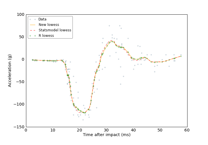
The aggregate difference between R’s lowess and mine?

print 'R and New Lowess MAD: %5.2e' %
np.mean(np.abs(r_lowess['y'] - new_lowess[:, 1]))


R and New Lowess MAD: 1.62e-13

So it looks like it works.

Now let’s look at some timings. I’ll create some test data: 10,000 points, where x is uniformly distributed on [0, 20], and y = sin(x) + N(0, 0.5).

Statsmodel’s lowess:

%timeit -n 3 smlw.lowess(y, x)


3 loops, best of 3: 22.8 s per loop

The new Cythonized lowess:

%timeit -n 3 cyl.lowess(y, x)


3 loops, best of 3: 10.8 s per loop

This is without the delta trick. Skimming the fat off of those tight-looped operations and Cythonizing them cut the run time in half. 11 seconds still sucks, though, so let’s see what delta gets us.

delta = (x.max() - x.min()) \* 0.01
%timeit -n 3 cyl.lowess(y, x, delta = delta)


3 loops, best of 3: 125 ms per loop

Much better. That’s the kind of time skipping 36,000 weighted least-squares calculations will save you. Given that this is some curvy data, is all this linear interpolation acceptable? I’ll re-run both with a better level of the frac parameter; the default is 2/3, but I’ll reduce it to 1/10 to use smaller neighborhoods in the regression and allow for more curvature. Here’s the plot:

sm_lowess = smlw.lowess(y, x, frac = 0.1)
new_lowess = cyl.lowess(y, x, frac = 0.1, delta = delta)

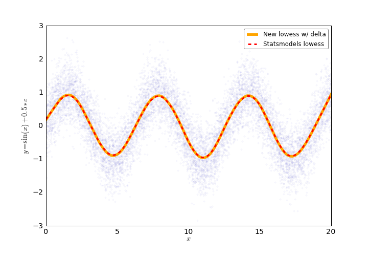
Which looks just as good as the non-interpolated version, but doesn’t leave you twiddling your thumbs.

Conclusion

After all this, we have a version of lowess that’s competitive with R’s lowess function. R also has a much richer loess function, for which there’s no real statmodels equivalent. loess is a full-blown class from which one can make predictions and compute confidence intervals, among other things. It also allows for fitting a higher-dimensional surface, not just a curve. But I have a day job, so that’s all for some other time. This kind of simple lowess is typically enough for most needs.

With this obsessive compulsive diversion into the guts of lowess out of the way, I’ll wrap up Chapter 2 of MLFH in my next post.