The code for Chapter 8 has been sitting around for a long time now. Let’s blow the dust off and check it out. One thing before we start: explaining PCA well is kinda hard. If any experts reading feel like I’ve described something imprecisely (and have a better description), I’m very open to suggestions.

Introduction

Chapter 8 is about Principal Components Analysis (PCA), which the authors perform on data with time series of prices for 24 stocks. In very broad terms, PCA is about projecting many real-life, observed variables onto a smaller number of “abstract” variables, the principal components. Principal components are selected in order to best preserve the variation and correlation of the original variables. For example, if we have 100 variables in our data, which are all highly correlated, we can project them down to just a few principal components—-i.e., the high correlation between them can be imagined as coming from an underlying factor that drives all of them, with some other less important factors driving their differences. When variables aren’t highly correlated, more principal components are needed to describe them well.

As you might imagine, PCA can be a very effective way of dealing with multi-collinearity that crops up in datasets with lots of variables. The downside is that PCA is just a mechanical process that is independent of the phenomenon we’re studying; the “principal components” we find don’t have to have any real-world meaning—-they’re just mathematical constructs. Sometimes we can give meaningful interpretations to the principal components by analogizing them to real underlying factors that theoretically drive our data. But this can be tricky, from both a technical and epistemological standpoint.

For the stocks the authors analyze, they ultimately try and reduce their description to a single principal component, which they interpret as a kind of “market-wide” factor, and compare with a broad market index (here the DJIA). This is a not uncommon application of PCA in stock analysis. But they’ve got a technical problem here.

To perform PCA, your data have to have a meaningful covariance matrix (or correlation matrix, but the conditions are equivalent). They analyze stock prices, which are non-stationary time series variables. This means their covariance matrices change with time, so you can’t really estimate a meaningful covariance matrix from a sample of data. Your estimator implicitly assumes the data are stationary, so your estimated covariance matrix is meaningless. If we calculate the stock returns in the data, though, we can do PCA properly, and we’ll see the relationship of the resulting principal component with the broad market index is much cleaner.

If you’re comfortable with PCA already, you don’t really have to worry about the conceptual content of this chapter. If you’re not, my advice it to take this chapter as a decent toy example of where and why one uses PCA, but don’t apply what’s done here elsewhere without learning more first. I’m not going to explain PCA in any detail; I just want to show where PCA functions live in the Python ecosystem and how they work. But, like most machine learning techniques, it shouldn’t be used at home without adult supervision.

As usual the IPython notebook lives at the Github repo here, and can be viewed via nbviewer here.

Stock data munging

The raw data are in a long format, with (no. of stocks) × (no. of days) rows, and three columns (a date, a stock ticker and a price for that ticker on that day). This sort of dataset lends itself to a pandas DataFrame with a hierarchical index—and since there’s only one variable in the data (the price), we’ll squeeze the DataFrame to get a Series. The Dow Jones data, containing just one ticker, is more straightforward.

prices_long = read_csv('data/stock_prices.csv', index_col = [0, 1],
                       parse_dates = True, squeeze = True)
dji_all = read_csv('data/dji.csv', index_col = 0, parse_dates = True,
                   squeeze = True)

With the stock data indexed this way, it’s easy to create a date × ticker DataFrame with prices as entries—-we just use unstack.

prices = prices_long.unstack()

Since we’ll ultimately want to perform this analysis with price returns, I’m going to create a similar dataset, just with returns instead of prices (note this will have one less day of data, since we don’t know the return for the first day in the data).

calc_returns = lambda x: np.log(x / x.shift(1))[1:]
returns = prices.apply(calc_returns)

Note I’m using log returns here. Pandas DataFrames have a pct_change method that would provide another way of computing returns.

The authors’ PCA strategy here is to extract a “stock index” factor from the stock data by using the first principal component—-this is the single principal component that captures the most variation in the underlying data.

The function make_pca_index is going to extract this first principal component, using the PCA function in scikit-learn’s sklearn.decomposition module. This is not the only way to get a PCA in Python—-indeed PCA is mechanically just an eigen-decomposition of the data’s correlation or covariance, so you could do this all from scratch in Numpy. The scikit-learn implementation, though, gives us a convenient PCA object to work with. And as usual with scikit-learn, the documentation is very good.

The PCA function works with a covariance or correlation matrix. We’re going to use a correlation matrix here; and our function will just take either stock price or return data, compute its correlation, then find the first principal component of the data. Notice the sign change I do at the end there—-the component ended up being negatively related to the data (i.e. when this factor goes down, the data go up, etc.). PCA results are typically sign- and scale-invariant; hence the problems with interpretation. We’ll make our resulting index a “postive” one by just reversing the sign.

def make_pca_index(data, scale_data = True):
    '''
    Compute the correlation matrix of a set of stock data, and return
    the first principal component.

    By default, the data are scaled to have mean zero and variance one
    before performing the PCA.
    '''
    if scale_data:
        data_std = data.apply(scale)
    else:
        data_std = data
    corrs = np.asarray(data_std.cov())
    pca   = PCA(n_components = 1).fit(corrs)
    # We end up getting a negative value for the index, so we'll reverse
    # the sign to have it be more intuitive.
    mkt_index = -scale(pca.transform(data_std))
    return mkt_index

A PCA index with price data

Let’s copy the authors and make an index from raw price data. Since prices don’t have meaningully-estimated correlations, this isn’t really correct, but it’s useful to compare with what’s in the book.

price_index = make_pca_index(prices)

To see what’s going on, let’s make two plots: a scatter plot of our PCA index with the DJIA, and a time series plot with the two indices. These correspond to figures 8-4 and 8-5 in the book.

plt.figure(figsize = (17, 5))
plt.subplot(121)
plt.plot(price_index, scale(dji), 'k.')
plt.xlabel('PCA index')
plt.ylabel('Dow Jones Index')
ols_fit = OLSreg(scale(dji), price_index)
plt.plot(price_index, ols_fit.fittedvalues, 'r-',
         label = 'R2 = %4.3f' % round(ols_fit.rsquared, 3))
plt.legend(loc = 'upper left')
plt.subplot(122)
plt.plot(dates, price_index, label = 'PCA Price Index')
plt.plot(dates, scale(dji), label = 'DJ Index')
plt.legend(loc = 'upper left')

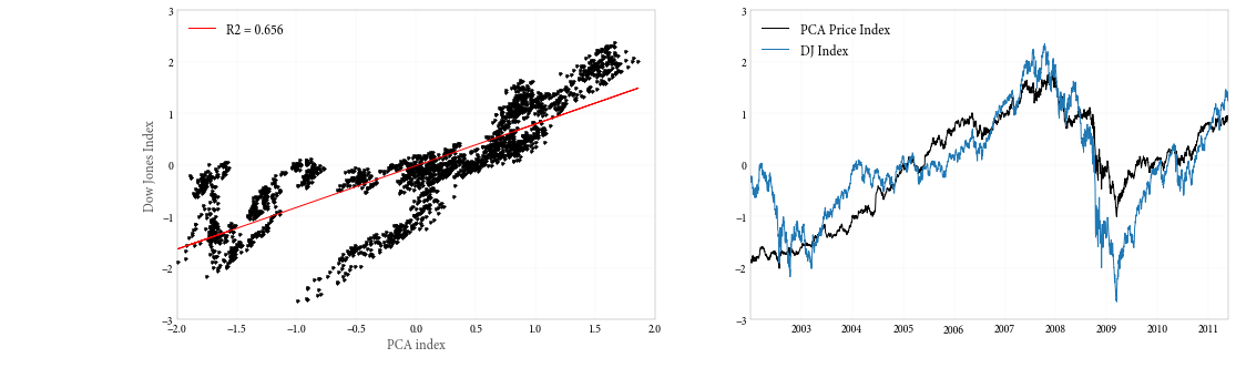
This actually seems to look okay, and wouldn’t really alert us to any problems if we didn’t know any better. Let’s repeat the exercise with returns, though.

A PCA index with returns data

Since returns are stationary, we can estimate a meaningful correlation matrix, and our PCA will make more sense.

returns_index = make_pca_index(returns)

And the plots:

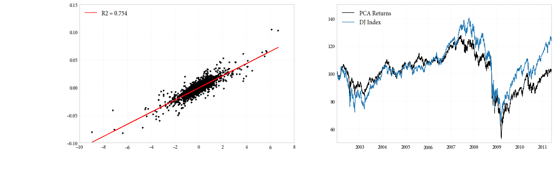
Looking at these, we see a much more straightforward linear relationship between the returns to the DJIA and the PCA index derived from stock returns.

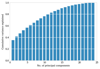
Explained variance

Since the principal components are just eigenvalues, there will be as many of them as their are columns in our data (here 24). As we add components we explain more and more of the original correlation matrix. Once we add all 24 the amount of variation/correlation explained is 100%—-all we’ve done is define a rotation of the matrix, so there’s no information lost. But a plot of the cumulative explained variance as we add principal components can help us to see how far and how reliably the data can be reduced.

plt.bar(arange(24) + .5, pca_fit.explained_variance_ratio_.cumsum())
plt.ylim((0, 1))
plt.xlabel('No. of principal components')
plt.ylabel('Cumulative variance explained')
plt.grid(axis = 'y', ls = '-', lw = 1, color = 'white')

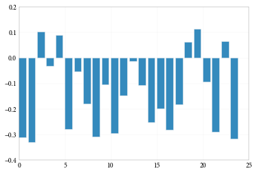
Factor loadings

We can also check out the loadings of the principal component across the stocks. What this shows us is how a change in the relates to the stocks in our data. For example a a component going up might cause half the stock returns in the data to go up and half to go down (it would positively load on some and negatively load on others.) We would expect, intuitively, a factor representing “the market,” as we think our first component does, to load on our stocks in the same direction, and roughly the same magnitude. And this is basically what we see.

plt.bar(arange(24), pca_fit.components_[0])

Conclusion

Since PCA is such a widely-used and fundamental technique, it’s important to know how to do it in Python, and the scikit-learn implementation is a good one. Check out the documentation here. Of course, like any statistical technique, PCA can definitely be misused, or at least easily misintepreted, so handle with care.