Introduction

This post will wrap up Chapter 1 of MLFH. The only task left is to replicate the authors’ trellis graph on p. 26. The plot is made up of 50 panels, one for each U.S. state, with each panel plotting the number of UFO sightings by month in that state.

The key takeaways from this part are, unfortunately, a bunch of gripes about Matplotlib. Since I can’t transmit, blogospherically, the migraine I got over the two afternoons I spent wrestling with this graph, let me just try to succinctly list my grievances.

1. Out-of-the-box, Matplotlib graphs are uglier than those produced by either lattice or ggplot in R: The default color cycle is made up of dark primary colors. Tick marks and labels are poorly placed in anything but the simplest graphs. Non-data graph elements, like bounding boxes and gridlines, are too prominent and take focus away from the data elements.
2. The API is deeply confusing and difficult to remember. You have various objects that live in various containers. To make adjustments to graphs, you have to remember what container the thing you want to adjust lives in, remember what the object and its property is called, and then remember how Matplotlib’s getting and setting procedures work.
3. The pyplot set of commands is supposed to provide convenience functions, but these abstractions seem to leak early and often. Once you need to make finer adjustments, you’re back to the underlying API nightmare.
4. The documentation is both clear and comprehensive. But where it is clear, it is not comprehensive, and where it is comprehensive, it is not clear. For example, the Artist tutorial is a pretty clear big picture of Matplotlib’s API. Once you need any detail, though, you’re dealing with this.
5. Creating trellis graphs requires way more manual work than in either lattice or ggplot. The supblot functionality of Matplotlib is highly flexible, but in most cases, the user is going to want the code to do the thinking for them and not manually place every graph (or do a bunch of bookkeeping with loops).

With that off my chest, let me say that I have a ton of respect for Matplotlib’s developers. It is a massively complex library, and clearly very powerful and flexible. I have no doubt that Matplotlib gurus can do amazing things. I’m just trying to convey the non-guru’s perspective. Graphing libraries are difficult to design because they must be incredibly flexible and allow users to manipulate all of the myriad parts of the graph, but at the same time, they can’t overwhelm users with detail when the flexibility isn’t needed. How anyone does it–especially in an open-source project–I don’t know.

It’s also possible that I’m just Doing it Wrong, and in fact there are easy ways to do all the things I’ve complained about. If that’s the case, I hope someone reading this will enlighten me.

Trellis graphs in R and Matplotlib

In my opinion, trellis graphs are the “killer app” of multivariate data visualization. I produce trellis line and scatter plots more than almost any other kind of visualization. As such, it’s important for me to be able to easily produce quality trellis graphs.

Trellis graphs are easy to create in R. The two most popular high-level graphing packages in R, lattice and ggplot, both have simple methods for creating them. Indeed, creating trellis graphs is lattice’s raison d’etre, and the functionality and interface design in the package revolves around dealing with trellis graph and the panels within. In ggplot, the trellis is not such a central focus, but it still has easy-to-use methods for making and modifying trellis graphs (which it refers to as “faceted” graphs).

For example, the graph we want to make is a one liner in lattice:

xyplot(sightings ~ year_month | us_state, data = sightings_counts,
type = 'l', layout = c(5, 10))

Once you get the hang of R’s formula expressions–which doesn’t take long–this is an easy, expressive way to create a trellis graph. The authors use ggplot, which I find a bit less natural, but is still very easy.

Part of what makes trellis graphs to straightforward in R is that the concept of factors, and their use as conditioning variables, is so well-baked into the language. Matplotlib is essentially a plotting utility for NumPy, so it’s designed to plot arrays, not rich data structures. Without factors, without a notion of conditioning, and to a lesser extent, without formulas, trellis graphs just don’t come naturally.

Pandas, though, has structures that, if a plotting library was designed to understand them, might provide for easy trellis-ing. Even though Pandas doesn’t have factors, I could see, for example, a plot method for Pandas’ groupby objects that produces trellis graphs by default.

Plotting the UFO trellis graph

With all that throat-clearing out of the way, let’s get down to plotting the graph. The authors plot 50 state panels, with a 10-by-5 layout. Since I’ve included D.C. in my data, I have to plot 51 panels. You can fit this in a 17-by-3 layout, but that’s pretty awkward. I’d like to have 4 columns instead, but to fit 51 graphs, I’ll need 13 columns. That’s 52 subplots, meaning the 13th row won’t have graphs in every column, only the first three. I’m going to call these last three graphs the hangover graphs, and I’m going to define it as its own variable to help inform the layout procedures I run later.

Here are the layout parameters, then:

nrow = 13; ncol = 4; hangover = len(us_states) % ncol[/sourcecode]

Now let me get the “framing” objects in place: the figure, the subplot layout, and the titles.

fig, axes = plt.subplots(nrow, ncol, sharey = True,
figsize = (9, 11))

fig.suptitle('Monthly UFO Sightings by U.S. State\nJanuary 1990 through August 2010',
             size = 12)
plt.subplots_adjust(wspace = .05, hspace = .05)

The subplots function is some recently-implement syntactic sugar around Matplotlib’s subplot functionality (see the section on “Easy Pythonic Subplots” here). The sharey argument tells Matplotlib that the panels should all share the same y axis. Technically I want it to share an x axis too, but Matplotlib kept throwing errors when I tried to use the sharex argument with dates on the x-axis. Give the data, the panels will end up sharing an x axis anyway, so this argument isn’t necessary. The function returns two objects: fig refers to the overall figure container, and axes is an array containing each of the subplot/panel objects – so axes[0, 0] is the first panel.

Now the rest of the code:

num_state = 0
for i in range(nrow):
for j in range(ncol):
xs = axes[i, j]

xs.grid(linestyle = '-', linewidth = .25, color = 'gray')

if num_state < 51:
    st = us_states[num_state]
    sightings_counts.ix[st, ].plot(ax = xs, linewidth = .75)
    xs.text(0.05, .95, st.upper(), transform = axes[i, j].transAxes,
    verticalalignment = 'top')
    num_state += 1
else:
    # Make extra subplots invisible
    plt.setp(xs, visible = False)

xtl = xs.get_xticklabels()
ytl = xs.get_yticklabels()

# X-axis tick labels:
# Turn off tick labels for all the the bottom-most
# subplots. This includes the plots on the last row, and
# if the last row doesn't have a subplot in every column
# put tick labels on the next row up for those last
# columns.
#
# Y-axis tick labels:
# Put left-axis labels on the first column of subplots,
# odd rows. Put right-axis labels on the last column
# of subplots, even rows.
if i < nrow - 2 or (i < nrow - 1 and (hangover == 0 or j <= hangover - 1)):
    plt.setp(xtl, visible = False)
if j > 0 or i % 2 == 1:
    plt.setp(ytl, visible = False)
if j == ncol - 1 and i % 2 == 1:
    xs.yaxis.tick_right()

plt.setp(xtl, rotation=90.)

Let’s walk through this:

First, set up a counter to keep track of what state we’re plotting. This is a little un-Pythonic, but given what I do inside the loop, I couldn’t think of a better way.

Now, for each row, column in the 13-by-4 array of panels (and this code works for any row/column combination, as long as rows × columns >= 51):

1. Assign the panel (“axis”) associated with this row, column pair to its own variable.
2. Draw gray gridlines in the panel.
3. Go to the state in the us_state list corresponding to the current value of the state counter.
4. Select this state out of the sightings_counts series and plot its data in the current panel. Then, put a text label with the state’s initials in the upper left corner.
5. If I’ve gone through all the states, and the state counter variable is greater than 51, then make the panel invisible.
6. Assign the x- and y-axis ticklabel objects for the current panel to variables. We’re going to manipulate their attributes.

7. Now some tricky stuff. I want do the following things to the tick labels:

   • I want to turn off the x-axis tick labels for all but the bottom-most panels, taking into account the hangover.
   • I want to alternate the y-axis tick labels so that they are on the left for odd-numbered rows, and on the right for even-numbered rows. Having labels on both sides makes the graph easier to read, but having them on the same side on every row leads to overcrowding and overlapping.

8. Finally, I want the x-axis tick labels rotated 90 degrees. This gives space to put as many as possible on the graph without overcrowding (here, we can label every two years).

Here’s the result:

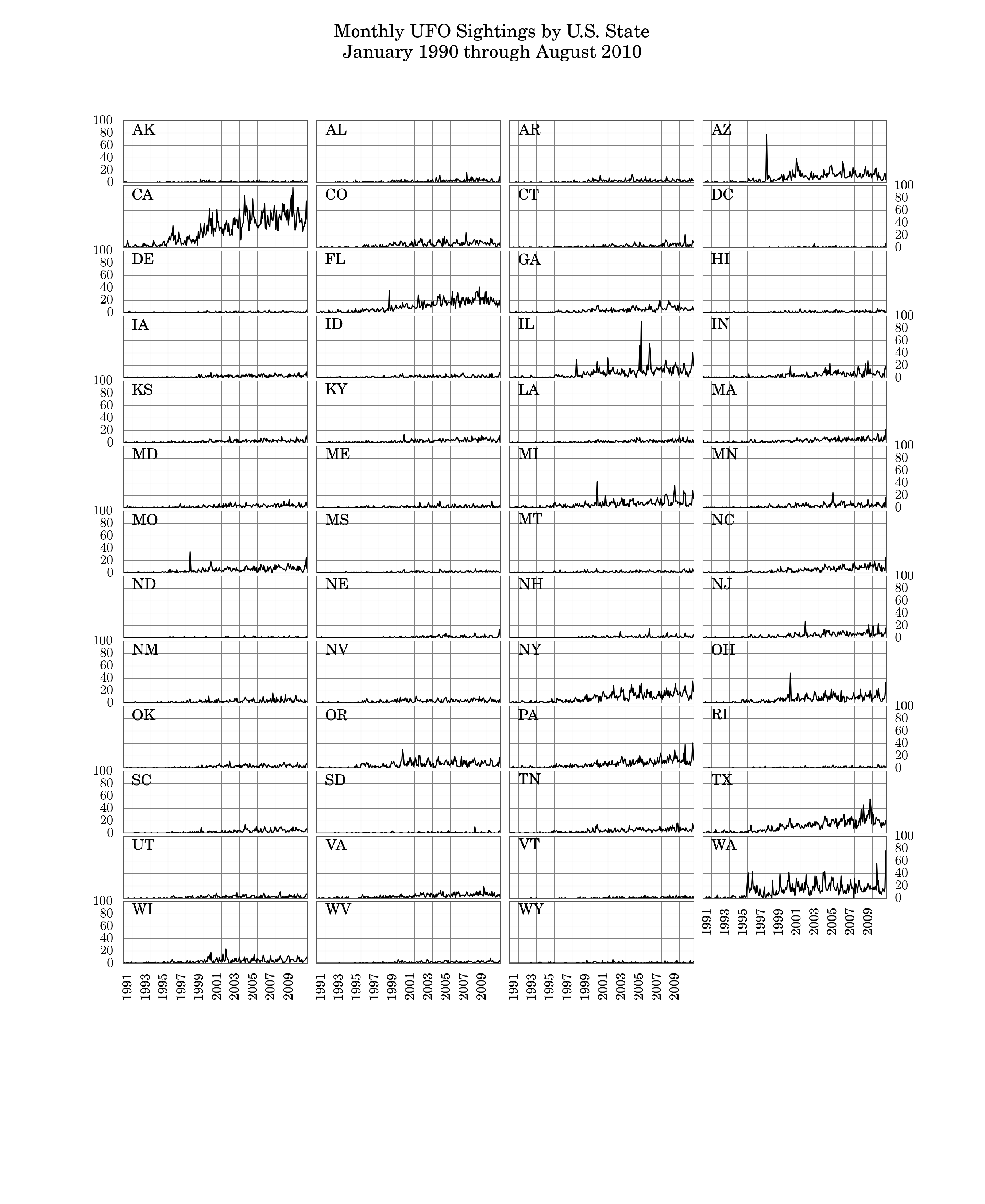
Not bad, I think. And maybe even better than the out-of-the-box version you get with ggplot. But it was a tremendous amount of work, and I don’t know if I’m going to be able to decipher this code six months from now. It’s just a tremendous amount of bookkeeping I have to do keeping track of what panel I’m in and where it’s located in the layout. There ought to be a function that does this for me.

Conclusion

So that’s it for Chapter 1 of MLFH. Overall, I was pleasantly surprised by Pandas and how easy it made loading, cleaning, and manipulating data. While there are a couple of things from R that I missed, there were several other things I though were easier and more flexible with Pandas.

On the other hand, going from lattice and ggplot to Matplotlib is like taking a time machine back to the early ‘90s. After reading the documentation and experimenting for several days, I still don’t think I’m sure how it works. Hopefully I’ll get the hang of it as I go forward.

My take is the Python data analysis community is aware of its “visualization gap” vis-a-vis R, and there are tools in the works to solve this issue. I’ve heard whispers about “ggplot for Python” or “D3 for Python.” Everything is still in the early stages, and it will probably be a while before better tools are available.

I’m also a little uncertain about the “x for Python” notion of creating graphing libraries. Matplotlib’s pyplot is essentially a “Matlab for Python” approach to graphics, and I don’t know that works to its credit. I’d much rather have a solid, Pythonic graphing library that lets me easily make publication-quality versions of the workhorse data graphics, than have something that apes the latest faddish graphing tool. There are a lot of smart people working on the problem, though, and I’m really excited to see what happens.