ARM Chapter 5: Logistic models of well-switching in Bangladesh
The logistic regression we ran for chapter 2 of Machine Learning for Hackers was pretty simple. So I wanted to find an example that would dig a little deeper into statsmodels’s capabilities and the power of the patsy formula language.
So, I’m taking an intermission from Machine Learning for Hackers and am going to show an example from Gelman and Hill’s Data Analysis Using Regression and Multilevel/Hierarchical Models (“ARM”). The chapter has a great example of going through the process of building, interpreting, and diagnosing a logistic regression model. We’ll end up with a model with lots of interactions and variable transforms, which is a great showcase for patsy and the statmodels formula API.
Logistic model of well-switching in Bangladesh
Our data are information on about 3,000 respondent households in Bangladesh with wells having an unsafe amount of arsenic. The data record the amount of arsenic in the respondent’s well, the distance to the nearest safe well (in meters), whether that respondent “switched” wells by using a neighbor’s safe well instead of their own, as well as the respondent’s years of education and a dummy variable indicating whether they belong to a community association.
  switch arsenic      dist assoc educ
1      1    2.36 16.826000     0    0
2      1    0.71 47.321999     0    0
3      0    2.07 20.966999     0   10
4      1    1.15 21.486000     0   12
5      1    1.10 40.874001     1   14
...
Our goal is to model well-switching decision. Since it’s a binary variable (1 = switch, 0 = no switch), we’ll use logistic regression.
The IPython notebook is at the Github repo here, and you can go here to view it on nbviewer. The analysis follows ARM chapter 5.4.
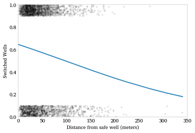
Model 1: Distance to a safe well
For our first pass, we’ll just use the distance to the nearest safe
well. Since the distance is recorded in meters, and the effect of one
meter is likely to be very small, we can get nicer model coefficients if
we scale it. Instead of creating a new scaled variable, we’ll just do it
in the formula description using the I() function.
model1 = logit('switch ~ I(dist/100.)', df = df).fit()
print model1.summary()
Optimization terminated successfully. Current function value: 2038.118913 Iterations 4 Logit Regression Results
==============================================================================
Dep. Variable: switch No. Observations: 3020
Model: Logit Df Residuals: 3018
Method: MLE Df Model: 1
Date: Sat, 22 Dec 2012 Pseudo R-squ.: 0.01017
Time: 13:05:25 Log-Likelihood: -2038.1
converged: True LL-Null: -2059.0
LLR p-value: 9.798e-11

==================================================================================
coef std err z P>|z| [95.0% Conf. Int.]

----------------------------------------------------------------------------------
Intercept 0.6060 0.060 10.047 0.000 0.488 0.724
I(dist / 100.) -0.6219 0.097 -6.383 0.000 -0.813 -0.431
Let’s plot this model. We’ll want to jitter the switch data, since
it’s all 0/1 and will over-plot.
Another way to look at this is to plot the densities of distance for switchers and non-switchers. We expect the distribution of switchers to have more mass over short distances and the distribution of non-switchers to have more mass over long distances.

Model 2: Distance to a safe well and the arsenic level of own well
Next, let’s add the arsenic level as a regressor. We’d expect respondents with higher arsenic levels to be more motivated to switch.
model2 = logit('switch ~ I(dist / 100.) + arsenic', df = df).fit()
print model2.summary()


Optimization terminated successfully.
Current function value: 1965.334134
Iterations 5
Logit Regression Results

==============================================================================
Dep. Variable: switch No. Observations: 3020
Model: Logit Df Residuals: 3017
Method: MLE Df Model: 2
Date: Sat, 22 Dec 2012 Pseudo R-squ.: 0.04551
Time: 13:05:29 Log-Likelihood: -1965.3
converged: True LL-Null: -2059.0
LLR p-value: 1.995e-41

==================================================================================
coef std err z P>|z| [95.0% Conf. Int.]

----------------------------------------------------------------------------------
Intercept 0.0027 0.079 0.035 0.972 -0.153 0.158
I(dist / 100.) -0.8966 0.104 -8.593 0.000 -1.101 -0.692
arsenic 0.4608 0.041 11.134 0.000 0.380 0.542

==================================================================================
Which is what we see. The coefficients are what we’d expect: the farther to a safe well, the less likely a respondent is to switch, but the higher the arsenic level in their own well, the more likely.
Marginal Effects
To see the effect of these on the probability of switching, let’s calculate the marginal effects at the mean of the data.
model2.margeff(at = 'mean')
array([-0.21806505, 0.11206108])
So, for the mean respondent, an increase of 100 meters to the nearest safe well is associated with a 22% lower probability of switching. But an increase of 1 in the arsenic level is associated with an 11% higher probability of switching.
Class separability
To get a sense of how well this model might classify switchers and non-switchers, we can plot each class of respondent in (distance-arsenic)-space. We don’t see very clean separation, so we’d expect the model to have a fairly high error rate. But we do notice that the short-distance/high-arsenic region of the graph is mostly comprised switchers, and the long-distance/low-arsenic region is mostly comprised of non-switchers.

Model 3: Adding an interaction
It’s sensible that distance and arsenic would interact in the model. In other words, the effect of an 100 meters on your decision to switch would be affected by how much arsenic is in your well.
Again, we don’t have to pre-compute an explicit interaction variable. We
can just specify an interaction in the formula description using the :
operator.
model3 = logit('switch ~ I(dist / 100.) + arsenic + I(dist / 100.):arsenic',
df = df).fit()
print model3.summary()


Optimization terminated successfully.
Current function value: 1963.814202
Iterations 5
Logit Regression Results

==============================================================================
Dep. Variable: switch No. Observations: 3020
Model: Logit Df Residuals: 3016
Method: MLE Df Model: 3
Date: Sat, 22 Dec 2012 Pseudo R-squ.: 0.04625
Time: 13:05:33 Log-Likelihood: -1963.8
converged: True LL-Null: -2059.0
LLR p-value: 4.830e-41

==========================================================================================
coef std err z P>|z| [95.0% Conf. Int.]

------------------------------------------------------------------------------------------
Intercept -0.1479 0.118 -1.258 0.208 -0.378 0.083
I(dist / 100.) -0.5772 0.209 -2.759 0.006 -0.987 -0.167
arsenic 0.5560 0.069 8.021 0.000 0.420 0.692
I(dist / 100.):arsenic -0.1789 0.102 -1.748 0.080 -0.379 0.022

==========================================================================================
The coefficient on the interaction is negative and significant. While we can’t directly intepret its quantitative effect on switching, the qualitative interpretation gels with our intuition. Distance has a negative effect on switching, but this negative effect is reduced when arsenic levels are high. Alternatively, the arsenic level have a positive effect on switching, but this positive effect is reduced as distance to the nearest safe well increases.
Model 4: Adding education, more interactions, and centering variables
Respondents with more eduction might have a better understanding of the harmful effects of arsenic and therefore may be more likely to switch. Education is in years, so we’ll scale it for more sensible coefficients. We’ll also include interactions amongst all the regressors.
We’re also going to center the variables, to help with interpretation of the coefficients. Once more, we can just do this in the formula, without pre-computing centered variables.
model_form = ('switch ~ center(I(dist / 100.)) + center(arsenic) + ' +
              'center(I(educ / 4.)) + ' +
              'center(I(dist / 100.)) : center(arsenic) + ' +
              'center(I(dist / 100.)) : center(I(educ / 4.)) + ' +
              'center(arsenic) : center(I(educ / 4.))'
             )
model4 = logit(model_form, df = df).fit()
print model4.summary()


Optimization terminated successfully.
Current function value: 1945.871775
Iterations 5
Logit Regression Results

==============================================================================
Dep. Variable: switch No. Observations: 3020
Model: Logit Df Residuals: 3013
Method: MLE Df Model: 6
Date: Sat, 22 Dec 2012 Pseudo R-squ.: 0.05497
Time: 13:05:35 Log-Likelihood: -1945.9
converged: True LL-Null: -2059.0
LLR p-value: 4.588e-46

===============================================================================================================
coef std err z P>|z| [95.0% Conf. Int.]

---------------------------------------------------------------------------------------------------------------
Intercept 0.3563 0.040 8.844 0.000 0.277 0.435
center(I(dist / 100.)) -0.9029 0.107 -8.414 0.000 -1.113 -0.693
center(arsenic) 0.4950 0.043 11.497 0.000 0.411 0.579
center(I(educ / 4.)) 0.1850 0.039 4.720 0.000 0.108 0.262
center(I(dist / 100.)):center(arsenic) -0.1177 0.104 -1.137 0.256
-0.321 0.085
center(I(dist / 100.)):center(I(educ / 4.)) 0.3227 0.107 3.026 0.002
0.114 0.532
center(arsenic):center(I(educ / 4.)) 0.0722 0.044 1.647 0.100 -0.014
0.158

===============================================================================================================
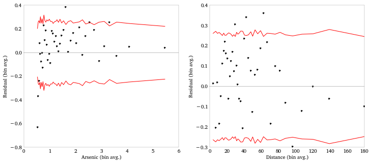
Model assessment: binned residual plots
Plotting residuals to regressors can alert us to issues like nonlinearity or heteroskedasticity. Plotting raw residuals in a binary model isn’t usually informative, so we do some smoothing. Here, we’ll averaging the residuals within bins of the regressor. (A lowess or moving average might also work.)
I’m going to write a function to provide the binned residual data
dynamically (and another helper function to plot the data). To create
the bins I’m going to use the handy qcut function in pandas, which
bins a vector of data into quantiles. Then I’ll use groupby to
calculate the bin means and confidence intervals.
def bin_residuals(resid, var, bins):
    '''
    Compute average residuals within bins of a variable.

    Returns a dataframe indexed by the bins, with the bin midpoint,
    the residual average within the bin, and the confidence interval
    bounds.
    '''
    resid_df = DataFrame({'var': var, 'resid': resid})
    resid_df['bins'] = qcut(var, bins)
    bin_group = resid_df.groupby('bins')
    bin_df = bin_group['var', 'resid'].mean()
    bin_df['count'] = bin_group['resid'].count()
    bin_df['lower_ci'] = -2 * (bin_group['resid'].std() /
    np.sqrt(bin_group['resid'].count()))
    bin_df['upper_ci'] = 2 * (bin_group['resid'].std() /
    np.sqrt(bin_df['count']))
    bin_df = bin_df.sort('var')
    return(bin_df)

def plot_binned_residuals(bin_df):
    '''
    Plotted binned residual averages and confidence intervals.
    '''
    plt.plot(bin_df['var'], bin_df['resid'], '.')
    plt.plot(bin_df['var'], bin_df['lower_ci'], '-r')
    plt.plot(bin_df['var'], bin_df['upper_ci'], '-r')
    plt.axhline(0, color = 'gray', lw = .5)

    arsenic_resids = bin_residuals(model4.resid, df['arsenic'], 40)
    dist_resids = bin_residuals(model4.resid, df['dist'], 40)
    plt.figure(figsize = (12, 5))
    plt.subplot(121)
    plt.ylabel('Residual (bin avg.)')
    plt.xlabel('Arsenic (bin avg.)')
    plot_binned_residuals(arsenic_resids)
    plt.subplot(122)
    plot_binned_residuals(dist_resids)
    plt.ylabel('Residual (bin avg.)')
    plt.xlabel('Distance (bin avg.)')
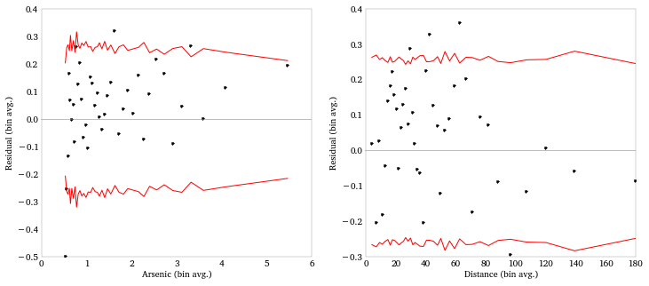
Model 5: log-scaling arsenic
The binned residual plot indicates some nonlinearity in the arsenic variable. Note how the model over-estimated for low arsenic and underestimates for high arsenic. This suggests a log transformation or something similar.
We can again do this transformation right in the formula.
model_form = ('switch ~ center(I(dist / 100.)) +
               center(np.log(arsenic)) + ' +
              'center(I(educ / 4.)) + ' +
              'center(I(dist / 100.)) : center(np.log(arsenic)) + ' +
              'center(I(dist / 100.)) : center(I(educ / 4.)) + ' +
              'center(np.log(arsenic)) : center(I(educ / 4.))'
             )

model5 = logit(model_form, df = df).fit()
print model5.summary()


Optimization terminated successfully.
Current function value: 1931.554102
Iterations 5
Logit Regression Results

==============================================================================
Dep. Variable: switch No. Observations: 3020
Model: Logit Df Residuals: 3013
Method: MLE Df Model: 6
Date: Sat, 22 Dec 2012 Pseudo R-squ.: 0.06192
Time: 13:05:57 Log-Likelihood: -1931.6
converged: True LL-Null: -2059.0
LLR p-value: 3.517e-52

==================================================================================================================
coef std err z P>|z| [95.0% Conf. Int.]

------------------------------------------------------------------------------------------------------------------
Intercept 0.3452 0.040 8.528 0.000 0.266 0.425
center(I(dist / 100.)) -0.9796 0.111 -8.809 0.000 -1.197 -0.762
center(np.log(arsenic)) 0.9036 0.070 12.999 0.000 0.767 1.040
center(I(educ / 4.)) 0.1785 0.039 4.577 0.000 0.102 0.255
center(I(dist / 100.)):center(np.log(arsenic)) -0.1567 0.185 -0.846
0.397 -0.520 0.206
center(I(dist / 100.)):center(I(educ / 4.)) 0.3384 0.108 3.141 0.002
0.127 0.550
center(np.log(arsenic)):center(I(educ / 4.)) 0.0601 0.070 0.855 0.393
-0.078 0.198

==================================================================================================================
And the binned residual plot for arsenic now looks better.
Model error rates
The pred_table() gives us a confusion matrix for the model. We can use
this to compute the error rate of the model.
We should compare this to the null error rates, which comes from a model that just classifies everything as whatever the most prevalent response is. Here 58% of the respondents were switchers, so the null model just classifies everyone as a switcher, and therefore has an error rate of 42%.
print model5.pred_table()
print 'Model Error rate: {0: 3.0%}'.format(
    1 - np.diag(model5.pred_table()).sum() / model5.pred_table().sum())
print 'Null Error Rate: {0: 3.0%}'.format(1 - df['switch'].mean())

[[ 568. 715.]
[ 387. 1350.]]
Model Error rate: 36%
Null Error Rate: 42%
Conclusion
So this was a more in-depth example of running a logistic regression with statsmodels and the formula API. Unlike last time, when we were just specifying the variables in the model, here we used the formula language to apply transforms and create interactions. I really love this: it drastically reduces the number of steps between thinking up a model and fitting it.
Comments